1. Denotational semantics and observations

This talk is about characterizing the preorder on λ-terms induced by a model — the relational semantics — as an operationally defined contextual preorder.

We’ll see that the relational semantics corresponds to a quantitative improvement order.

1.1. Operational semantics

Reduction relation: \[ M \rightarrow N~\text{and its transitive closure}~M \rightarrow^{*} N \]

Use this to define a notion of observation \(\obs{M}\).

Examples:

• \(M \rightarrow^* 0\) in some typed language with constants
• \(M \rightarrow^* \mathsf{hnf}\) (aka \(M\) is solvable in untyped λ-calculus)

From this we define a contextual preorder: \(M \lectx N\) means \[ \text{for all contexts}~C[-]. \obs{C[M]} \subseteq \obs{C[N]} \]

1.2. Denotational semantics

Interpret programs as mathematical entities:

for a program phrase \(M\), its interpretation is \(\sem{M}\).

Typically \(\sem{M}\) is some kind of function

• continuous functions between complete partial orders
• homomorphisms of some algebraic structure

We’ll mostly consider the case where \(\sem{M}\) is a relation.

Other kinds of models exist, e.g. game semantics.

1.3. Denotational preorder

If the universe of interpretations carries a natural partial order, we obtain a denotational preorder on programs: \[ M \leden N \Leftrightarrow \sem{M} \sqsubseteq \sem{N}. \]

1.4. Observations in denotational semantics

Typically, denotational models also allow us to make “observations”: for example

• denotational evaluation to values e.g. \(0 \in \sem{M}\)
• denotational definedness: \(\sem{M} \not = \perp\)

We usually expect that the denotational partial order preserves observations i.e. \[ \sem{M} \sqsubseteq \sem{N} \Rightarrow \obs{\sem{M}} \subseteq \obs{\sem{N}}. \]

1.5. Operational/denotational correspondence properties

1.5.1. Observational soundness

\[ \obs{M} \subseteq \obs{\sem{M}} \]

Typically easy to prove. It sometimes follows readily from reduction invariance \[ M \rightarrow N \quad \Rightarrow \quad \sem{M} = \sem{N}. \] plus simple facts about the semantics of normal forms.

1.5.2. Computational adequacy

\[ \obs{\sem{M}} \subseteq \obs{M}. \]

This says that the operational semantics is adequate to generate all observations predicted by the model.

1.5.3. Inequational soundness

\[ M \leden N \Rightarrow M \lectx N. \]

This follows from the observational soundness and adequacy properties, provided the denotational semantics is compositional and monotone.

1.5.4. Completeness

\[ M \lectx N \Rightarrow M \leden N \]

This property is notoriously difficult to establish for many kinds of programming language. For PCF this is the famous full abstraction problem.

In the λ-calculus, the situation is different.

2. Lambda calculus and Böhm trees

\[ M ::= x \mid MM \mid \lambda x.M \quad\quad (\lambda x.M)N \rightarrow_\beta M[N/x] \]

In the pure λ-calculus there is another important class of preorders based on Böhm-trees.

If \(M\rightarrow^* \lambda x_{1}\ldots x_{n}.y\,M_{1}\cdots M_{k}\):

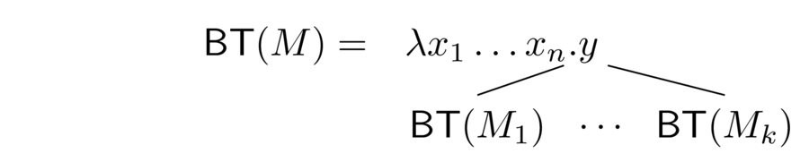
Otherwise, \(M\) is head diverging: \( \BT{M} = \bot.\)

2.1. Bohm preorder

3. Böhm preorder up to extensionality

We also define two extensions:

• \(M \sqsubseteq_{\mathbf{B}\eta} N\) means that the Böhm tree of \(M\) is contained in that of \(N\) up to η-conversion
• \(M \sqsubseteq_{\mathbf{B}\eta^{\text{red}}} N\) means that the Böhm tree of \(M\) is contained in that of \(N\) up to η-reduction

\[ x \not \sqsubseteq_{\mathbf{B}} \lambda y. xy \quad \lambda y. xy \not \sqsubseteq_{\mathbf{B}} x \] \[ x \sqsubseteq_{\mathbf{B}\eta} \lambda y. xy \quad \lambda y. xy \sqsubseteq_{\mathbf{B}\eta} x \] \[ x \not \sqsubseteq_{\mathbf{B}\eta^{\text{red}}} \lambda y. xy \quad \lambda y. xy \sqsubseteq_{\mathbf{B}\eta^{\text{red}}} x \]

3.1. \(D_\infty\) models

In the standard domain-theoretic models of λ-calculus – the so-called \(D_\infty\) models – we have the correspondence \[ \sem{M} \not = \bot \Leftrightarrow M\rightarrow^*\mathsf{hnf}. \]

Taking a contextual preorder based on observing reduction to head normal form, we get \[ M \leden N \Rightarrow M \lectx N. \]

We also have \[ M \sqsubseteq_{\mathbf{B}\eta} N \Rightarrow M \leden N. \]

The “Böhm-out” technique (Hyland (1976)) builds contexts that distinguish terms with distinct Böhm-trees: \[ M \not \sqsubseteq_{\mathbf{B}\eta} N \Rightarrow \exists C[-]. C[M] \rightarrow^*\mathsf{hnf}~\text{but}~C[N]\not\rightarrow^*\mathsf{hnf} \]

Therefore \[ \sem{M} \sqsubseteq \sem{N} \Leftrightarrow M \lectx N. \]

4. Relational semantics

This talk is about the relational semantics of the λ-calculus.

Relational semantics grew from Girard’s quantitative semantics (1988) and can be seen as a simple model of linear logic (Girard, 1987).

4.1. A Cartesian closed category of relations

Our model will interpret programs as certain kinds of relations. They can be seen as morphisms of a cartesian closed category defined by:

• objects: sets
• morphisms \(A\rightarrow B\): relations from \(\mathbf{M}_f(A)\) to \(B\)

Here \(\mathbf{M}_f(A)\) is the set of finite multisets drawn from \(A\).

The model is a reflexive object in this category.

However, the model is easier to explain in the form of a non-idempotent intersection type system.

4.2. Relational semantics as a type system

Idea: give a system of type derivations yielding judgements of the form \[ x_1: \mu_1, \ldots, x_n:\mu_n \vdash M: \alpha \] The denotation of a term is the set of its valid typings.

In this case, each “type” \(\mu_i\) is a multiset of types, so we get something akin to the morphisms in the category described above.

4.3. Intersection types

\[ \frac{}{x:[\alpha] \vdash x:\alpha}~\text{ax} \quad\quad \frac{\Gamma_i \vdash M: \alpha_i~~(i \in I~\text{finite})}{\uplus_{i \in I}\Gamma_i \vdash M: [\alpha_i]_{i \in I}}~\text{many} \]

\[ \frac{\Gamma, x:\mu \vdash M: \alpha}{\Gamma \vdash \lambda x.M: \mu \rightarrow \alpha}~\lambda \quad\quad \frac{\Gamma \vdash M: \mu \rightarrow \alpha \quad \Delta \vdash N: \mu} {\Gamma \uplus \Delta \vdash MN : \alpha}~\text{@} \]

4.4. Facts about the type system

• A term may have many types: the types are elements of the denotational semantics rather than traditional types
• A term in head normal form trivially has a type. For example \[ x: [] \rightarrow [] \rightarrow a \vdash x M N : a \] Note that a term such as \( x \Omega\) has a type, though \(\Omega\) does not.
• Subject reduction and expansion hold

4.5. Subject reduction / expansion

If \( M \rightarrow_\beta N \) then \[ \Gamma \vdash M: \alpha \Leftrightarrow \Gamma \vdash N:\alpha \]

Taking \(\sem{M}\) to be the set of typings of \(M\), this says: \[ \text{if}~M\rightarrow_\beta N~\text{then}~\sem{M} = \sem{N}. \]

4.6. Quantitative aspects

This model has quantitative content: the multisets count something. But what?

They keep track of how many times an argument is used: for example we can type \[ f: [[\alpha] \rightarrow [\alpha'] \rightarrow \alpha] \vdash \lambda x. f~x~x:[\alpha, \alpha']\rightarrow \alpha. \]

The many rule means that these multiplicities are also seen in derivations. \[ \cfrac{\cfrac{\vdots}{f: [[\alpha] \rightarrow [\alpha'] \rightarrow \alpha] \vdash \lambda x. f~x~x:[\alpha, \alpha']\rightarrow \alpha}\quad \cfrac{\vdash M: \alpha \quad \vdash M: \alpha'}{\vdash M: [\alpha,\alpha']}}{f: [[\alpha] \rightarrow [\alpha'] \rightarrow \alpha]\vdash (\lambda x. f~x~x) M: \alpha }~@ \] The function uses \(M\) twice, so we need two derivations of \(M\).

Though substitution may duplicate or discard terms, it does not duplicate or discard their type derivations.

4.7. Quantitative subject reduction

Type derivations track more quantitative information than the types: a typing of \((\lambda x. M)N\) contains exactly one more @-rule than the matching typing of \(M[N/x]\).

So for head reductions \[ \lambda x_1 \ldots x_n. R~M_1 \ldots M_k \rightarrow_h \lambda x_1 \ldots x_n. R'~M_1 \ldots M_k \] we have a quantitative subject reduction theorem.

The restriction to head reductions is essential : for example \(x \Omega \rightarrow_\beta x \Omega\), but this is never a head reduction.

4.8. Understanding the relational preorder

We now know: \[ \text{if}~\sem{M} \subseteq \sem{N}~\text{then for all}~C[-]. C[M]\rightarrow^* \mathsf{hnf} \Rightarrow C[N]\rightarrow^* \mathsf{hnf}\] and hence the denotational order implies the extensional Böhm-tree order \[ M \sqsubseteq_{\mathbf{B}\eta} N\]

The converse is not true. For example \(x \sqsubseteq_{\mathbf{B}\eta} \lambda y. x y \) but \[ x : [a] \vdash x: a \quad\quad x : [a] \not\vdash \lambda y. x y: a \quad \]

In fact thanks to Breuvart, Manzonetto and Ruoppolo (2018) we know that

• \(\sem{M} \subseteq \sem{N}\) ⇔ \(M \sqsubseteq_{\mathbf{B}\eta^{\text{red}}} N\)

But these are all qualitative. Where have the quantities gone? Can we recover a contextual ordering by paying attention to quantities?

5. Improvement orders

Sands introduced the idea of a contextual improvement order.

Idea: observe not just what happens but how long it takes.

For example: observe the length of a head-reduction sequence.

We write \( M \Downarrow^k \) if \(M\) reduces to hnf in \(k\) head reduction steps.

Then we can define improvement: \(M \leimp N \) iff \[ \text{for all contexts}~C[-]. C[M]\Downarrow^k \Rightarrow \exists k'\leq k. C[N]\Downarrow^{k'} \]

\(N\) does the same things as \(M\) in fewer steps.

Note that an order that counts reductions cannot be the order induced by a denotational semantics that is sound for beta-reduction.

(There are very few denotational models of improvement orders as a result. One exception is Ghica’s slot games (2005)).

So our plan to use this idea to capture the relational order must fail. Yet here we are…

6. Checkers calculus

Accattoli et al. (2025) introduced the checkers calculus.

Idea: distinguish internal reductions of a term from interactions with its context.

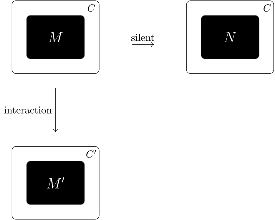
6.1. Checkers syntax

Terms are labelled with two badges: \(\bullet\) for “internal” and \(\circ\) for “external”. \[ M, N ::= x \mid \lambda_\bullet x. M \mid \lambda_\circ x. M \mid M \bullet N \mid M \circ N \]

Silent reductions: \[ (\lambda_\bullet x.M)\bullet N \rightarrow M[N/x] \quad (\lambda_\circ x.M)\circ N \rightarrow M[N/x] \]

Interaction reductions: \[ (\lambda_\bullet x.M)\circ N \stackrel{\interact}{\rightarrow} M[N/x] \quad (\lambda_\circ x.M)\bullet N \stackrel{\interact}{\rightarrow} M[N/x] \]

We can embed the ordinary λ-calculus by using \(\bullet\) for every label. Every reduction would be silent.

The fun starts when we embed a \(\bullet\)-labelled term in a \(\circ\)-labelled context.

6.2. Example

Two versions of the identity function in the context \(- \circ (\lambda_\circ x.x) \).

Note that eta-expansion increases the number of interaction steps, and also changes the labelling of the result.

6.3. Checkers improvement ordering

We can now define an appropriate improvement ordering for terms of this calculus.

We observe the number of interaction steps in a head-reduction sequence.

We write \( M \Downarrow^k \) if \(M\) reduces to hnf in \(k\) head interaction steps.

Then we can define improvement: \(M \leimp N \) iff \[ \text{for all contexts}~C[-]. C[M]\Downarrow^k \Rightarrow \exists k'\leq k. C[N]\Downarrow^{k'} \]

\(N\) does the same things as \(M\) in fewer interaction steps.

For a regular λ-term labelled with \(\bullet\) throughout, all steps are silent.

Terms that are β-equivalent will be equivalent in this preorder.

But our example shows that \(\circ\)-labelled contexts can distinguish between η-convertible terms: η-reduction seems to deliver improvement.

Conjecture The interaction improvement preorder on λ-terms coincides with the relational preorder.

First step If \(M \leimp N\) then \(M \sqsubseteq_{\mathbf{B}\eta^{\text{red}}} N\) (and hence \(\sem{M} \subseteq \sem{N}\) in the relational semantics).

Proved via syntactic methods akin to Hyland’s Böhm-out technique.

For the converse we will refine the relational semantics.

7. Checkers semantics

We annotate the types:

and the judgements: \[ \Gamma \vdash^k M : \alpha \]

Judgement annotations track the number of interaction applications: \[ \frac{}{x:[\alpha] \vdash^0 x:\alpha}~\text{ax} \quad\quad \frac{\Gamma_i \vdash^{k_i} M: \alpha_i~~(i \in I~\text{finite})}{\uplus_{i \in I}\Gamma_i \vdash^{\sum_i k_i} M: [\alpha_i]_{i \in I}}~\text{many} \]

\[ \frac{\Gamma, x:\mu \vdash^k M: \alpha}{\Gamma \vdash^k \lambda_{\bullet/\circ} x.M: \mu \stackrel{\bullet/\circ}{\rightarrow} \alpha}~\lambda \]

\[ \frac{\Gamma \vdash^k M: \mu \stackrel{\bullet}{\rightarrow} \alpha \quad \Delta \vdash^{k'} N: \mu} {\Gamma \uplus \Delta \vdash^{k+k'} M \bullet N : \alpha}~\text{@-silent} \]

\[ \frac{\Gamma \vdash^k M: \mu \stackrel{\bullet}{\rightarrow} \alpha \quad \Delta \vdash^{k'} N: \mu} {\Gamma \uplus \Delta \vdash^{k+k'+1} M \circ N : \alpha}~\text{@-interact} \] (plus rules exchanging \(\bullet\) with \(\circ\)).

7.1. Examples

In the plain relational semantics we have the following typings for identity-like terms \[ \vdash \lambda x. x: [[a] \rightarrow a] \rightarrow [a] \rightarrow a \] \[ \vdash \lambda x. \lambda y. x y: [[a] \rightarrow a] \rightarrow [a] \rightarrow a \]

In the checkers calculus we have: \[ \vdash^0 \lambda_\bullet x. x : [[a] \stackrel{\bullet}{\rightarrow} a] \stackrel{\bullet}{\rightarrow} [a] \stackrel{\bullet}{\rightarrow} a \quad\quad \vdash^0 \lambda_\bullet x. \lambda_\bullet y. x \bullet y : [[a] \stackrel{\bullet}{\rightarrow} a] \stackrel{\bullet}{\rightarrow} [a] \stackrel{\bullet}{\rightarrow} a \] \[ \vdash^0 \lambda_\bullet x. x : [[a] \stackrel{\circ}{\rightarrow} a] \stackrel{\bullet}{\rightarrow} [a] \stackrel{\circ}{\rightarrow} a \quad\quad \vdash^1 \lambda_\bullet x. \lambda_\bullet y. x \bullet y : [[a] \stackrel{\circ}{\rightarrow} a] \stackrel{\bullet}{\rightarrow} [a] \stackrel{\bullet}{\rightarrow} a \] Key insight: η-reductions lead to typings that are either the same, or “whiter and cheaper”.

7.2. Correctness of the semantics

With the same techniques as for the regular relational semantics, we can prove

As a corollary, \[ \text{if}~\sem{M} \subseteq \sem{N}~\text{then}~M \leimp N. \]

However, semantic inclusion does not precisely capture \(\leimp\) because we know \[ \lambda_\bullet x. \lambda_\bullet y. x \bullet y \leimp \lambda_\bullet x. x \] We need to capture the “whiter and cheaper” idea.

7.3. Seeing improvements in typings

We write \(\alpha \leq_k^+ \alpha'\) if \(\alpha\) can be obtained from \(\alpha'\) by changing \(k\) positively occurring instances of \(\bullet\) to \(\circ\).

We write \(\alpha \leq_k^- \alpha'\) if \(\alpha\) can be obtained from \(\alpha'\) by changing \(k\) negatively occurring instances of \(\bullet\) to \(\circ\).

For example \[ [a] \stackrel{\circ}{\rightarrow} a \leq_1^+ [a] \stackrel{\bullet}{\rightarrow} a \] \[ [[a] \stackrel{\circ}{\rightarrow} a] \stackrel{\bullet}{\rightarrow} a \leq_1^- [[a] \stackrel{\bullet}{\rightarrow} a] \stackrel{\bullet}{\rightarrow} a \]

The typing of \(N\) is \(d\)-whiter and at least \(d\)-cheaper.

7.4. From the improvement order order to \(\lepwc\)

For ordinary λ-terms, we know \[ M \leimp N \Rightarrow M \sqsubseteq_{\mathbf{B}\eta^{\text{red}}} N \]

By direct analysis of typing derivations on Böhm-trees we can prove

It remains to prove that \(M \lepwc N\) implies \(M \leimp N\).

7.5. Is \(\lepwc\) compositional?

Suppose the \(\lepwc\) ordering is preserved by term constructors.

Then \(M \lepwc N\) implies \(C[M] \lepwc C[N]\) for any context \(C[-]\).

If \(C[M] \Downarrow^k\) then \(C[M]\) has a typing \(\vdash^k C[M] : \alpha\).

By \(\lepwc\) we obtain a typing \(\vdash^{k'} C[N]:\alpha'\) with \(k' \leq k\).

Hence \(C[N]\Downarrow^{k''}\) for some \(k'' \leq k' \leq k\).

So \(M \leimp N\).

But is \(\lepwc\) compositional?

7.6. The challenge of compositionality

Consider an application \[ \frac{\vdash^k M: [\alpha] \stackrel{\bullet}{\rightarrow} \beta \quad \vdash^{k'} N: \alpha}{\vdash^{k+k'} M \bullet N: \beta} \]

If we replace \(N\) by an improved (whiter-cheaper) term \[ \vdash^{k''} N': \alpha' \] where \(\alpha' \leq_d^+ \alpha\), we can no longer apply the rule.

We’d like to find a new typing for \(M\) of the form \[ \vdash^{l} M: [\alpha'] \stackrel{\bullet}{\rightarrow} \beta \]

7.7. Repainting typings

7.8. Repainting: propagation via variables

Start with \[ \vdash^0 \lambda_\bullet x. x : [[a] \stackrel{\bullet}{\rightarrow} a] \stackrel{\bullet}{\rightarrow} [a] \stackrel{\bullet}{\rightarrow} a \] Change a negatively occurring \(\bullet\) to \(\circ\): \[ \not\vdash^0 \lambda_\bullet x. x : [[a] \stackrel{\circ}{\rightarrow} a] \stackrel{\bullet}{\rightarrow} [a] \stackrel{\bullet}{\rightarrow} a \] Repainting a positively occurring \(\bullet\) to \(\circ\) yields a valid typing: \[ \vdash^0 \lambda_\bullet x. x : [[a] \stackrel{\circ}{\rightarrow} a] \stackrel{\bullet}{\rightarrow} [a] \stackrel{\circ}{\rightarrow} a \]

7.9. Repainting: propagation across applications

As we repaint a typing derivation, we may encounter \[ \frac{\vdash^k M: \mu \stackrel{\bullet}{\rightarrow} \alpha \quad \vdash^{k'} N: \mu}{\vdash^{k+k'} M\bullet N: \alpha} \] being repainted to \[ \frac{\vdash^k M: \mu \stackrel{\circ}{\rightarrow} \alpha \quad \vdash^{k'} N: \mu}{\not\vdash^{k+k'} M\bullet N: \alpha} \] The repainting here propagates to an additional interaction step: \[ \frac{\vdash^k M: \mu \stackrel{\circ}{\rightarrow} \alpha \quad \vdash^{k'} N: \mu}{\vdash^{k+k'+1} M\bullet N: \alpha} \]

7.10. Repainting: propagation back and forth

We may need to repaint more steps in the derivation: given \[ \frac{\vdash^k M: \mu \stackrel{\bullet}{\rightarrow} \alpha \quad \vdash^{k'} N: \mu}{\vdash^{k+k'} M\bullet N: \alpha} \] Repaint \(N:\mu\) to \(\mu' \leq_1^+ \mu\): \[ \frac{\vdash^k M: \mu \stackrel{\bullet}{\rightarrow} \alpha \quad \vdash^{k'} N: \mu'}{\not\vdash^{k+k'} M\bullet N: \alpha} \] repainting propagates to \(M\): \[ \frac{\not\vdash^k M: \mu' \stackrel{\bullet}{\rightarrow} \alpha \quad \vdash^{k'} N: \mu'}{\not\vdash^{k+k'} M\bullet N: \alpha} \] which requires repainting \(\mu'\) to \(\mu'' \leq_1^- \mu'\): \[ \frac{\vdash^k M: \mu'' \stackrel{\bullet}{\rightarrow} \alpha \quad \vdash^{k'} N: \mu'}{\not\vdash^{k+k'} M\bullet N: \alpha} \]

This is still not valid! But the process may terminate at the next step with e.g. \[ \frac{\vdash^k M: \mu'' \stackrel{\bullet}{\rightarrow} \alpha \quad \vdash^{k''} N: \mu''}{\vdash^{k+k''} M\bullet N: \alpha} \]

7.11. Termination of repainting

The termination argument is very easy:

• every non-final step changes one \(\bullet\) to \(\circ\) and does not change the type in any other way
• there are a finite number of annotations in a type

7.12. \(\lepwc\) is compositional

8. Summary

We introduced an interaction based improvement order on checkers terms, and hence on λ-terms.

We developed an annotated relational semantics and associated denotational improvement ordering \(\lepwc\).

On λ-terms, we showed that the order induced by the ordinary relational model coincides with the improvement order, yielding a quantitative analogue of the Hyland-Wadsworth theorem.

9. Bibliography